Proximal Policy Optimization Algorithms
PPO proposes a family of policy gradient methods that use a clipped surrogate objective to constrain policy updates, achieving the stability of trust-region methods (TRPO) with the simplicity of first-order optimization. Instead of solving a constrained optimization problem with second-order methods, PPO clips the importance sampling ratio to $[1-\epsilon, 1+\epsilon]$, preventing destructively large updates. Combined with Generalized Advantage Estimation and multiple epochs of minibatch updates, PPO delivers strong performance on continuous control (MuJoCo) and discrete (Atari) tasks. Published by OpenAI in 2017, PPO became the default RL optimizer for LLM alignment via RLHF — powering InstructGPT and ChatGPT.
Visualizations (11)
Abstract
The paper proposes a new family of policy gradient methods that alternate between sampling data through interaction with the environment and optimizing a "surrogate" objective function using stochastic gradient ascent.
- Gradient ascent is used since we want to maximize the reward (as opposed to gradient descent, which minimizes a loss).
- In RL, we try to maximize the expected cumulative reward.
- It's stochastic because you can't calculate the cumulative reward over all possible trajectories — only the sampled ones from the mini-batch.
Introduction
We want a method that is:
- Scalable — to large models and parallel implementations
- Data Efficient
- Robust — works on many problems without hyperparameter tuning
The landscape of existing approaches:
- Q-learning with function approximation fails on many simple problems and is poorly understood.
- TRPO is complicated — requires second-order optimization, conjugate gradients, and line search.
- Vanilla policy gradient methods are not data efficient or robust.
PPO achieves the stability of trust-region methods with the simplicity of first-order optimization. The proposed algorithm performs better than existing approaches on continuous control tasks.
Two Approaches to Learning a Policy
- Value-function based: Learn a value function that estimates "how good is each action in this state" and choose the action with the highest value. Only works well with discrete actions. Examples: Q-learning, DQN.
- Policy gradient: Parametrize the policy as a neural network that takes the state as input and outputs a probability distribution over actions. Use gradient ascent to adjust parameters so the policy produces actions that lead to higher rewards. Examples: REINFORCE, PPO, TRPO.
The distinction: "Which action is the best action?" (value function) vs "For this state, what should I do?" (policy gradient). However, policy gradient methods have high variance — you might get lucky, or not.
Background: Policy Gradient Methods
Policy gradient methods work by estimating the gradient of expected reward with respect to the policy parameters, then using stochastic gradient ascent to improve.
The most commonly used gradient estimator has the form:
where $\pi_\theta$ is a stochastic policy, $\widehat{A}_t$ is the estimator of the advantage function at timestep $t$, and $\widehat{\mathbb{E}}_t$ denotes an empirical average over a finite batch of samples.
In practice, automatic differentiation software constructs an objective function whose gradient is the policy gradient estimator:
Performing multiple steps of optimization on $L^{PG}$ using the same trajectory can lead to destructively large policy updates. This is the core problem PPO solves.
Intuition for the Method
You have a policy parametrized by a neural network ($\theta$). The policy maps states to action probabilities. You want to adjust $\theta$ so the policy collects more rewards.
The tricky part: the objective has an expectation over trajectories that depend on $\theta$ in a complex way:
How do you differentiate through this? Using the log-derivative trick:
This lets us rewrite the gradient of an expectation as an expectation we can sample:
The process becomes: run policy → collect trajectories → for each (state, action) pair compute reward × gradient → average across samples. This is the REINFORCE algorithm.
#1 Statistics Refresher
ManimAnimated review of key statistical concepts underpinning policy gradients: expectation, variance, log-derivative trick, and importance sampling.
#2 Policy Gradient Intuition
ManimVisual walkthrough of the REINFORCE algorithm: how actions with positive advantage get reinforced (probability increased) while actions with negative advantage get suppressed.
Derivation of the Policy Gradient Estimator
Setup
We have a parameterized policy $\pi_{\theta}(a_t|s_t)$ and want to maximize the expected return:
where $\tau = (s_0, a_0, s_1, a_1, \ldots)$ is a trajectory sampled under policy $\pi_{\theta}$.
Step 1: Probability of a trajectory
where $\rho(s_0)$ is the initial state distribution and $P(s_{t+1}|s_t,a_t)$ is the environment dynamics.
Step 2: Gradient of the objective
Step 3: The log-derivative trick
Using $\nabla_{\theta} P(\tau|\theta) = P(\tau|\theta) \cdot \nabla_{\theta} \log P(\tau|\theta)$:
Step 4: Simplify the log-trajectory probability
Taking the gradient w.r.t. $\theta$:
The initial state distribution and environment dynamics terms vanish — they don't depend on $\theta$. This is why policy gradients are model-free: we never need to know or differentiate through the environment dynamics.
Step 5: The REINFORCE gradient
Step 6: Introduce the advantage function
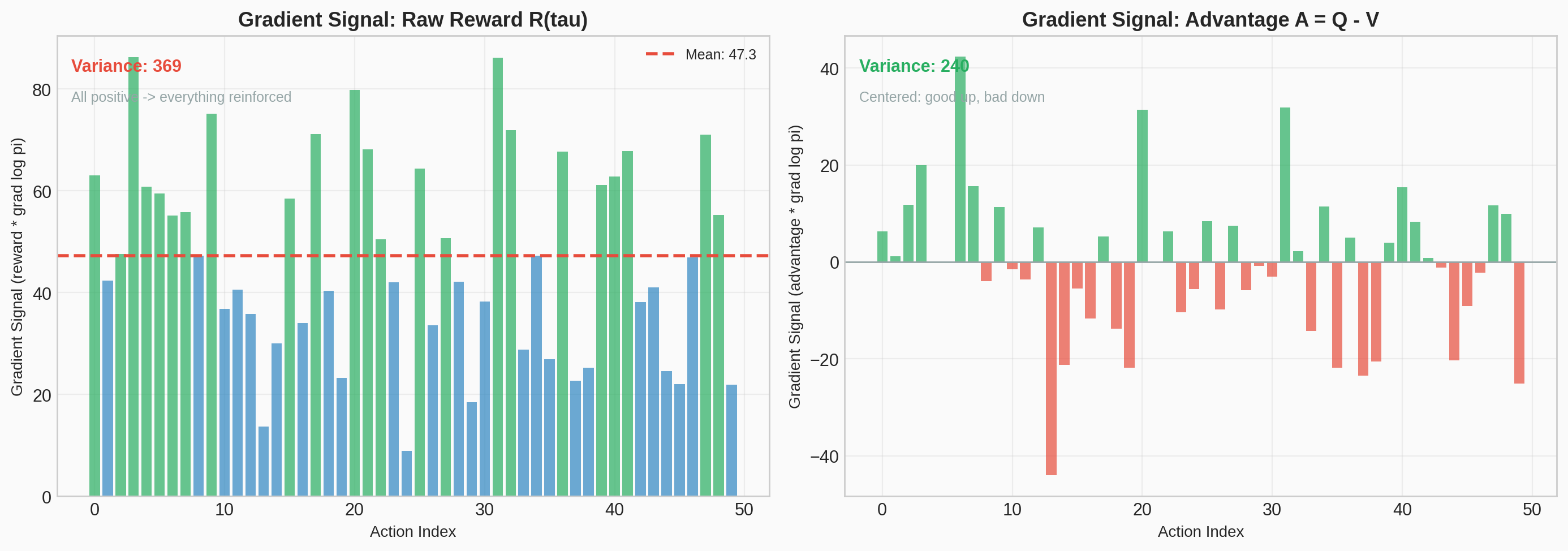
Using $R(\tau)$ produces high variance. Replace it with $\widehat{A}_t = Q(s_t, a_t) - V(s_t)$ without changing the expected gradient:
Step 7: The policy gradient estimator
Estimate this expectation by sampling and averaging:
where $\widehat{\mathbb{E}}_t$ denotes the empirical average over a finite batch of timesteps, and $\widehat{A}_t$ is an estimator of the advantage function (computed using GAE in PPO's case).
#3 Policy Gradient Derivation
ManimStep-by-step animated derivation of the policy gradient estimator, from trajectory probability through the log-derivative trick to the final REINFORCE formula.
The Advantage Function
Building Blocks
Value function $V(s_t)$ — "If I'm in state $s_t$ and follow my policy from here, what's my expected total future reward?"
Action-value function $Q(s_t, a_t)$ — "If I take specific action $a_t$ in state $s_t$, then follow my policy after that?"
Note that $V$ is just $Q$ averaged over all actions weighted by the policy: $V(s_t) = \sum_{a} \pi(a|s_t) \cdot Q(s_t, a)$.
Definition
"How much better (or worse) is this specific action compared to what I'd get on average from this state?"
- $A > 0$: this action is better than the average action from this state
- $A < 0$: this action is worse than average
- $A = 0$: this action is exactly as good as average
Why This Definition? — Variance Reduction
The "something" multiplying $\nabla_\theta \log \pi_\theta(a_t|s_t)$ in the policy gradient can be:
- Total trajectory reward $R(\tau)$ — valid but high variance
- Future reward from $t$ onward $\sum_{t' \geq t} r_{t'}$ — valid, lower variance
- $Q(s_t, a_t)$ — same expected gradient, focuses on the action's value
- $Q(s_t, a_t) - V(s_t)$ — same expected gradient, lowest variance
Rewards from the past can't influence future rewards, so past rewards just add variance. Looking at only the "rewards to go" ($Q$ from time $t$) removes that noise. Adding a state-dependent baseline ($V$) reduces variance even further — without introducing any bias.
Proof that subtracting $V(s_t)$ adds zero in expectation
Therefore subtracting $V(s_t)$ adds zero in expectation but dramatically reduces variance. The advantage is the optimal baseline for variance reduction in policy gradients.
Summary
By using gradient ascent with the advantage, we push up actions that have higher-than-average returns and push down those with lower-than-average returns. The advantage acts as both a filter and a multiplier.
#4 Advantage vs Raw Reward
Matplotlib PlotlySide-by-side comparison of policy gradient updates using raw trajectory rewards vs advantage-based estimation, showing how variance is reduced.
Static figure
Interactive demo — Open in new tab →
Generalized Advantage Estimation (GAE)
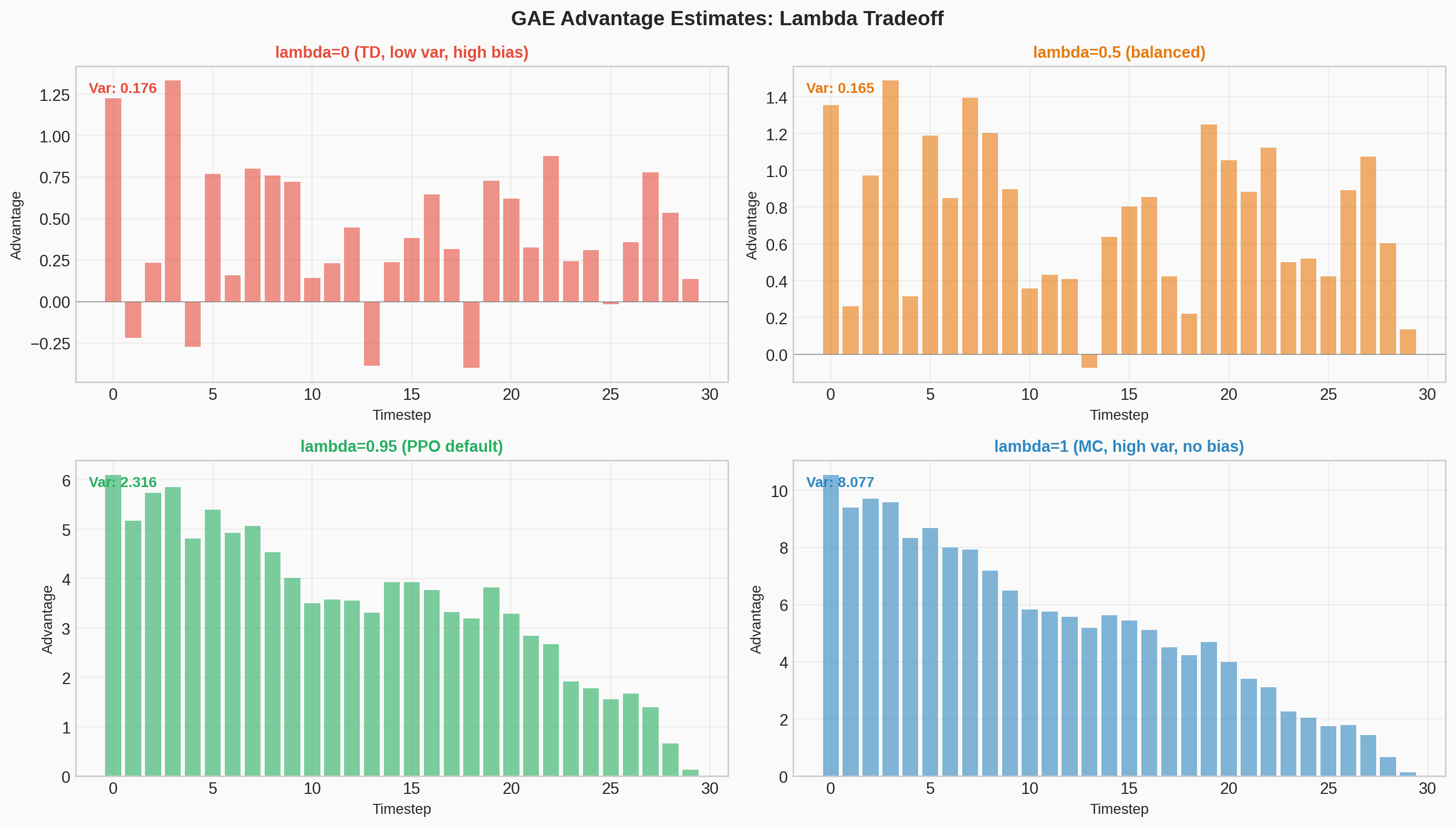
The $\widehat{A}_t$ in the PPO equation means "we don't know the true $A$, so we estimate it." PPO uses GAE, which introduces a parameter $\lambda$ that trades off bias and variance.
TD Residual
First, define the temporal difference (TD) residual at timestep $t$:
A one-step estimate of the advantage: "I got reward $r_t$, ended up in a state worth $V(s_{t+1})$, so the discounted value of what actually happened is $r_t + \gamma V(s_{t+1})$. Subtract what I expected, $V(s_t)$, to get the surprise."
The GAE Formula
where $\gamma \in [0, 1]$ is the discount factor and $\lambda \in [0, 1]$ controls the bias-variance tradeoff.
Special Cases
When $\lambda = 0$
Just the one-step TD residual. Low variance (only depends on one step of randomness) but high bias (relies entirely on $V$ being accurate).
When $\lambda = 1$
The full Monte Carlo return minus the baseline. No bias (uses actual rewards) but high variance (depends on the entire future trajectory).
$\lambda$ interpolates smoothly between these extremes. Instead of choosing between "trust your value function estimate" ($\lambda=0$) and "trust the raw Monte Carlo returns" ($\lambda=1$), GAE blends them. The $(\gamma\lambda)^l$ weighting means nearby TD residuals matter more and distant ones are exponentially downweighted. In practice, PPO typically uses $\lambda = 0.95$.
LLM connection: When PPO is used for LLM fine-tuning, each token generation is an action. Tokens with positive advantage (better than average continuations) get reinforced — made more likely — while tokens with negative advantage get suppressed.
#5 GAE Lambda Tradeoff
Matplotlib PlotlyInteractive visualization of how the GAE lambda parameter controls the bias-variance tradeoff in advantage estimation, with TD weight decay curves for different lambda values.
Static figure
Interactive demo — Open in new tab →
Trust Region Methods
In TRPO, the objective function ("surrogate objective") is maximized subject to a constraint on the size of the policy update.
The Fundamental Problem with Policy Gradients
The policy gradient gives us a direction to move $\theta$, but says nothing about how far to move:
The learning rate $\alpha$ is the problem. This is much worse than in supervised learning, for a reason specific to RL.
Why RL Is Different From Supervised Learning
In supervised learning, your dataset is fixed. A bad gradient step makes the loss go up, but next step you compute a gradient on the same data and recover.
In RL, your dataset is generated by your policy. A bad gradient step changes your policy, which changes what trajectories you collect, which changes the quality of your next gradient estimate.
This creates a feedback loop: bad update → bad policy → bad data → bad gradient → worse update → … A single overly large update can be unrecoverable. The policy enters a region of parameter space where it collects useless data, and no amount of subsequent gradient steps can fix it.
The Step Size Dilemma
- Small $\alpha$: safe but slow — you might need millions of updates.
- Large $\alpha$: fast but dangerous — risk the death spiral above.
- Adaptive methods (Adam, RMSProp) don't solve this. They adapt step sizes per-parameter, but have no notion of "how much did the policy change?"
The core insight: we don't care how much $\theta$ changes in Euclidean space. We care how much the policy distribution changes. A step of size 0.01 in $\theta$ might barely change the policy, or it might completely flip the action probabilities — depending on the local geometry.
#6 Trust Region Motivation
ManimAnimated comparison of parameter-space vs policy-space distances, showing how a small parameter change can cause a large policy shift and why KL-based trust regions are needed.
From Parameter Space to Distribution Space
We need a measure of distance between policies, not between parameter vectors. This is where KL divergence comes in:
KL divergence measures how different two probability distributions are. Always $\geq 0$, equals $0$ only when the distributions are identical. It is invariant to parametrization — even if the policy's parameters $\theta$ have changed a lot, it doesn't matter if the output distribution is similar.
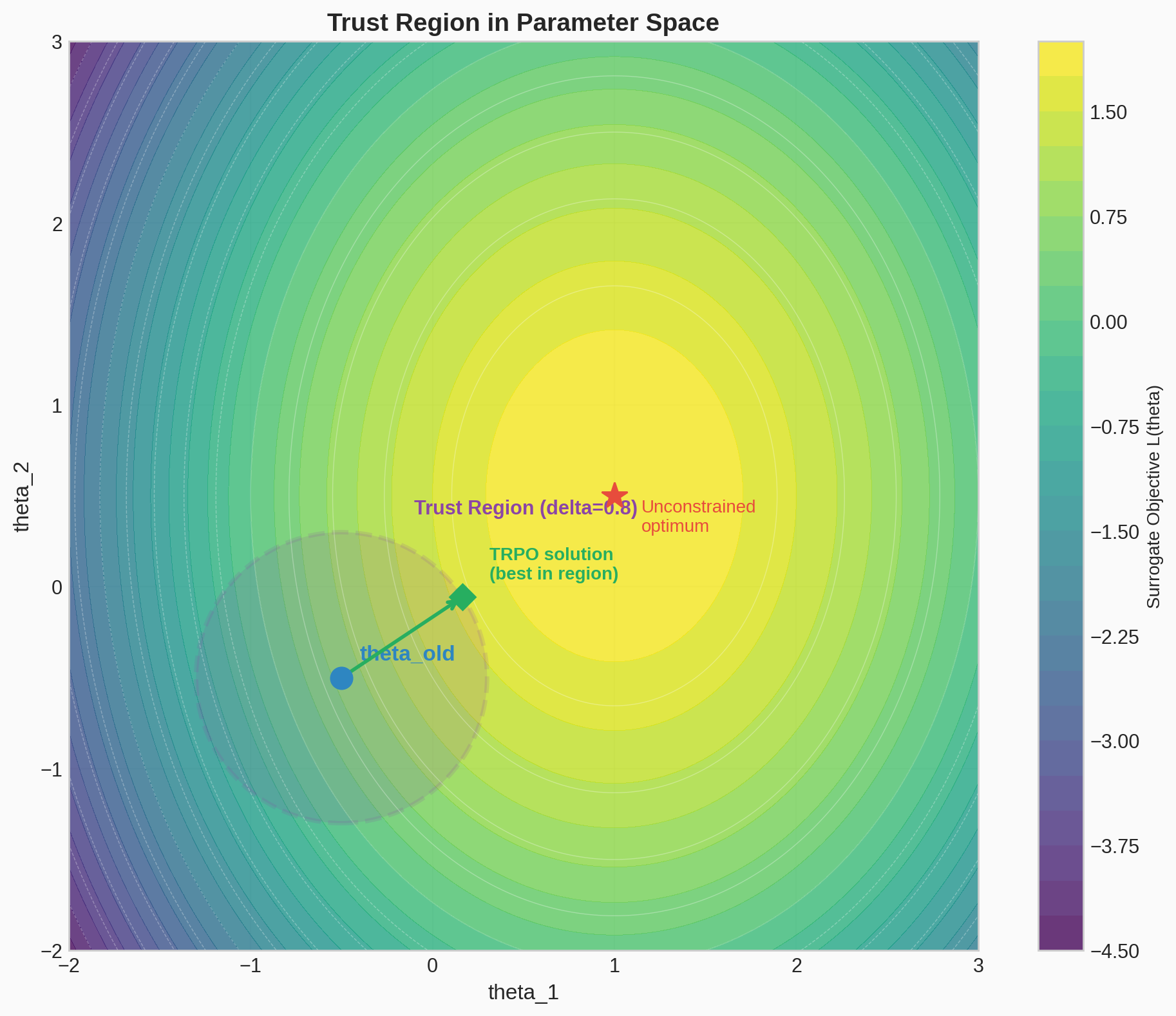
The Local Approximation (Surrogate Objective)
If $\pi_\theta$ is close to $\pi_{\theta_{\text{old}}}$, we can approximate the true objective by using importance sampling:
This surrogate is a good approximation only locally. Far from $\theta_{\text{old}}$, it breaks down because the state distribution diverges and the importance sampling ratio becomes unreliable.
TRPO: Constrained Optimization
TRPO formalizes "stay close" as:
The constraint defines a trust region — the set of all $\theta$ values where the KL divergence from the old policy is at most $\delta$. With a monotonic improvement guarantee.
The Cost of TRPO
Solving this constrained problem requires:
- Computing the Fisher information matrix $F$ (second-order derivative of KL w.r.t. $\theta$)
- Using conjugate gradient to approximately solve $F^{-1} g$
- A line search to find the largest step satisfying the KL constraint
This is doable but expensive and complex. This complexity is precisely what motivates PPO.
#7 KL Trust Region
Matplotlib PlotlyVisualization of the KL divergence constraint defining the trust region in policy space, showing how different constraint radii affect the allowed policy updates.
Static figure
Interactive demo — Open in new tab →
Clipped Surrogate Objective
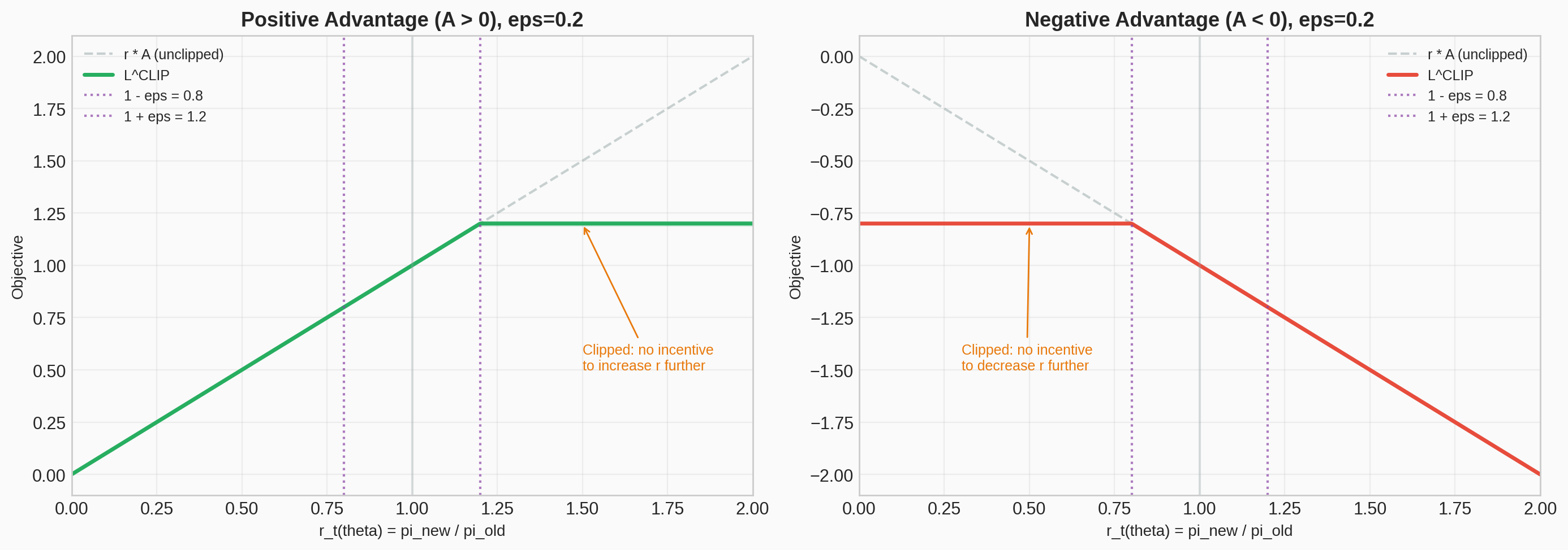
Define the probability ratio:
Without a constraint, maximizing $L^{CPI}(\theta) = \widehat{\mathbb{E}}_t [r_t(\theta)\widehat{A}_t]$ could lead to excessively large policy updates. PPO modifies the objective to penalize changes that move $r_t(\theta)$ away from 1:
where $\epsilon$ is a hyperparameter (typically $0.2$). By taking the minimum of the clipped and unclipped objective, the final objective is a pessimistic (lower) bound on the unclipped objective.
The motivation:
- The first term is the same as TRPO's surrogate.
- The second term clips the ratio, removing the incentive to move $r_t(\theta)$ outside $[1-\epsilon, 1+\epsilon]$.
- Where $r = 1$, both terms are equal. They diverge as $\theta$ moves away from $\theta_{\text{old}}$.
- The $\min$ handles both positive and negative advantages correctly.
When the advantage is positive ($A > 0$): the objective increases as $r$ increases (reinforcing the action), but clips at $1+\epsilon$ — preventing excessive reinforcement. When the advantage is negative ($A < 0$): the objective increases as $r$ decreases (suppressing the action), but clips at $1-\epsilon$ — preventing excessive suppression.
Adaptive KL Penalty (Alternative)
As an alternative to clipping, PPO can use an adaptive KL penalty:
The coefficient $\beta$ is adjusted dynamically:
- If $d < d_{\text{targ}} / 1.5$: update was too conservative, decrease $\beta \leftarrow \beta / 2$
- If $d > d_{\text{targ}} \times 1.5$: update was too aggressive, increase $\beta \leftarrow \beta \times 2$
In practice, this worked worse than the clipped surrogate objective.
The Progression
| Method | How it controls step size | Complexity |
|---|---|---|
| Vanilla PG | Fixed learning rate $\alpha$ | Simple, unstable |
| TRPO | Hard KL constraint, second-order optimization | Stable, complex |
| PPO (clip) | Clip importance ratio to $[1-\epsilon, 1+\epsilon]$ | Stable, simple |
| PPO (penalty) | Adaptive KL penalty in objective | Stable, simple |
The narrative arc: gradient direction is easy, step size is hard → step size in parameter space is the wrong thing to control → control distance in policy space instead (KL) → TRPO does this exactly but is complex → PPO approximates it simply.
#8 Clipped Surrogate Objective
Matplotlib PlotlyVisualization of the PPO clipping mechanism: how the surrogate objective is clipped for both positive and negative advantages, with the effective loss landscape.
Static figure
Interactive demo — Open in new tab →
Algorithm
Combined Loss
If the policy and value function share parameters (common in practice), the loss function combines the policy surrogate, a value function error term, and an entropy bonus:
where $c_1, c_2$ are coefficients, $S[\pi_\theta](s_t)$ is an entropy bonus to encourage exploration, and $L_t^{VF}(\theta) = ( V_\theta(s_t) - V_t^{\text{targ}} )^2$ is the squared-error value function loss.
Truncated GAE
The implementation runs the policy for $T$ timesteps (per trajectory segment, not per episode) and uses a truncated version of GAE:
PPO, Actor-Critic Style
Algorithm 1:
for iteration $= 1, 2, \ldots$ do
for actor $= 1, 2, \ldots, N$ do
Run policy $\pi_{\theta_{\text{old}}}$ in environment for $T$ timesteps
Compute advantage estimates $\widehat{A}_1, \ldots, \widehat{A}_T$
end for
Optimize surrogate $L$ w.r.t. $\theta$, with $K$ epochs and minibatch size $M \leq NT$
$\theta_{\text{old}} \leftarrow \theta$
end for
The algorithm is simple: collect a batch of experience with the current policy across $N$ parallel workers ($NT$ total timesteps). Compute advantages using GAE. Do $K$ passes of minibatch gradient ascent on the clipped surrogate. Snapshot the updated policy, throw away the batch, collect fresh data, and repeat. The clipping is what makes the $K$ epochs of reuse safe — without it, multiple passes over the same data would push the policy too far from where the data was collected.
#9 PPO vs TRPO vs PG
ManimAnimated comparison of vanilla policy gradient, TRPO, and PPO: showing how each method handles the step-size problem differently, with PPO achieving TRPO's stability via simple clipping.
Experiments
Comparison of Surrogate Objectives
- Tested clipping in log space — not much improvement.
- Used MuJoCo tasks with 1 million timesteps.
- Hyperparameters: $\epsilon$ (clip), $\beta$ (KL penalty), $d_{\text{targ}}$ (target KL).
- A 2-layer MLP with tanh activations was used. Policy and value function parameters were not shared, so the entropy bonus was not used.
Continuous Control (MuJoCo)
PPO outperformed on almost every task. To showcase performance on high-dimensional problems, the authors trained on 3D humanoid tasks: running, steering, getting up off the ground, and being pelted by cubes.
Atari
PPO achieved better results across Atari games as well. Some practitioners have used the adaptive KL variant for robotics applications.
The experiments confirmed that the clipped surrogate objective ($L^{CLIP}$) with $\epsilon = 0.2$ consistently matched or exceeded the performance of TRPO's constrained optimization — while being far simpler to implement and tune.
PPO for LLM Alignment
PPO became the standard RL algorithm for aligning language models via RLHF (Reinforcement Learning from Human Feedback). The connection:
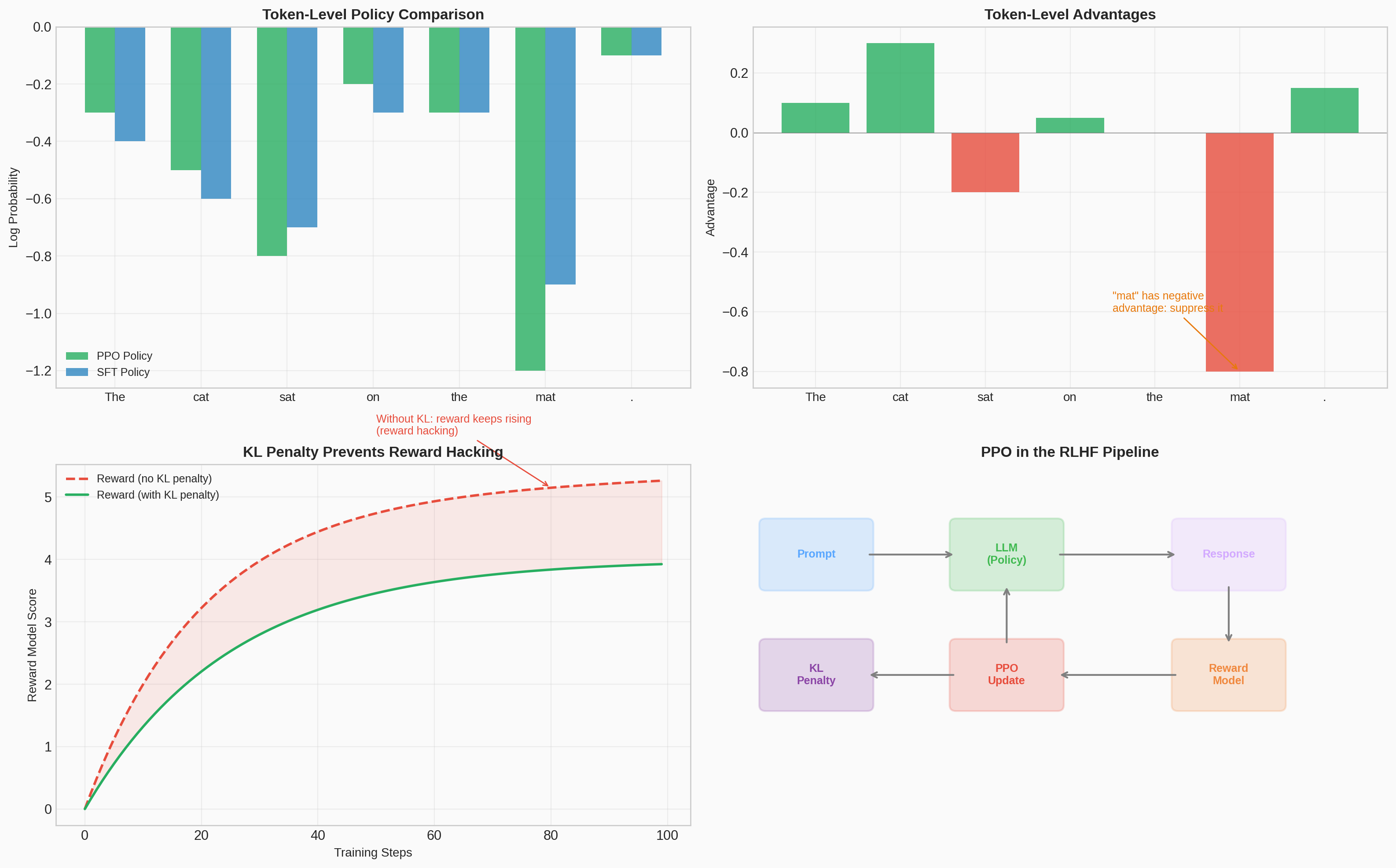
- Policy = the language model. Given a prompt (state), it generates tokens (actions).
- Reward model = trained from human preferences (as in the RLHF paper).
- PPO optimization = fine-tune the LM to maximize the learned reward while staying close to the original model (via KL penalty).
The KL penalty in LLM alignment serves the same purpose as PPO's clipping: prevent the model from diverging too far from the base policy. Without it, the model would "hack" the reward model by generating degenerate text that scores highly but is nonsensical. This is the same trust-region principle, applied at the token level.
This pipeline — pretrain LM, train reward model from preferences, fine-tune with PPO — powered InstructGPT (Ouyang et al., 2022) and ChatGPT. PPO's simplicity and stability made it the practical choice over TRPO for this application.
#10 PPO for LLM Alignment
Matplotlib PlotlyVisualization of how PPO is applied in the RLHF pipeline for language model alignment: the three-stage process from pretraining through reward modeling to PPO fine-tuning.
Static figure
Interactive demo — Open in new tab →
#11 Interactive CartPole Demo
Plotly/JSSelf-contained PPO implementation running in your browser: watch a simulated CartPole agent learn to balance a pole through clipped surrogate optimization. Adjust hyperparameters ($\epsilon$, $\gamma$, $\lambda$) and observe their effects in real time.
Interactive demo — Open in new tab →
Conclusion
Proximal Policy Optimization introduces a set of policy optimization methods that use stochastic gradient ascent to perform each policy update. These methods are as stable and reliable as trust-region methods, but simpler to implement, requiring only first-order optimization. Better overall performance across both continuous control and discrete action domains.
PPO's lasting impact goes beyond its original benchmarks. By making trust-region-quality RL optimization accessible to any practitioner with a standard deep learning toolkit, PPO became the backbone of LLM alignment — the algorithm that fine-tuned the models behind ChatGPT, Claude, and other instruction-following AI systems.